CNNs and Uncertainty Quantification
Introduction
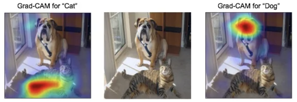
Using a Convolutional Neural Net (CNN), I determine whether the pictures are deer, frogs, or trucks. I design a Neural Net that includes three convolutional layers (they pick up on the structure in the picture) and feed the output into dense layers. The classification accuracy is just over 90%. Additionally, I apply Grad CAM to visualize which image structure led to the classification decision. Here is an example using a cat and a dog:
Convolutional Neural Network (CNN)
First, we build a CNN. We choose a batch size of 128, and specify that we are dealing with 3 classes. The CNN’s goal is to classify deers (0), frogs (1), and trucks (2) with an accuracy of >90%. The dimensions of the pictures are 32x32 and we use a softmax activation function in the final output layer for multicategorical classification. Moreover, note that these are color images. We use a validation split of 0.2.
# Data Preparation
batch_size <- 128
num_classes <- 3 #How many classes are we dealing with?
epochs <- 12

# Input image dimensions
img_rows <- 32 #use dim()
img_cols <- 32 #use dim()
input_shape <- c(img_rows, img_cols, 3) #3 because rbg image

#Build model and summary
model <- keras_model_sequential() %>%
  layer_conv_2d(filters = 32, kernel_size = c(3,3), activation = 'relu',
                input_shape = input_shape) %>%
  layer_max_pooling_2d(pool_size = c(2, 2)) %>%
  layer_conv_2d(filters = 64, kernel_size = c(3,3), activation = 'relu') %>%
  layer_max_pooling_2d(pool_size = c(2, 2)) %>%
  layer_conv_2d(filters = 128, kernel_size = c(3,3), activation = 'relu', name='Conv_last') %>%
  #Specifically named the last convolutional layer for Grad CAM later!
  layer_max_pooling_2d(pool_size = c(2, 2)) %>%
  layer_flatten() %>%
  layer_dense(units = 128, activation = 'relu') %>%
  layer_dropout(rate = 0.3) %>%
  layer_dense(units = 128, activation = 'relu') %>%
  layer_dropout(rate = 0.3) %>%
  layer_dense(units = num_classes, activation = 'softmax') #Classification: Softmax

summary(model)
| Layer (type) | Output Shape | Param # |
|---|---|---|
| conv2d_1 (Conv2D) | (None, 30, 30, 32) | 896 |
| max_pooling2d_2 (MaxPooling2D) | (None, 15, 15, 32) | 0 |
| conv2d (Conv2D) | (None, 13, 13, 64) | 18,496 |
| max_pooling2d_1 (MaxPooling2D) | (None, 6, 6, 64) | 0 |
| Conv_last (Conv2D) | (None, 4, 4, 128) | 73,856 |
| max_pooling2d (MaxPooling2D) | (None, 2, 2, 128) | 0 |
| flatten | (None, 512) | 0 |
| dense_2 (Dense) | (None, 128) | 65,664 |
| dropout_1 (Dropout) | ||
| dense_1 (Dense) | (None, 128) | 16,512 |
| dropout (Dropout) | ||
| dense (Dense) | (None, 3) | 387 |
Total params: 175,811
Trainable params: 175,811
Non-trainable params: 0
#Model compiling
model %>% compile(
  loss = 'categorical_crossentropy',
  optimizer = 'adam',
  metrics = c('accuracy')
)

#set up early stopping
callback_specs=list(callback_early_stopping(monitor = "val_loss", min_delta = 0, patience = 10,
                                            verbose = 0, mode = "auto"),
                    callback_model_checkpoint(filepath='best_model.hdf5',save_freq='epoch' ,save_best_only = TRUE)
)

#running optimization
history <- model %>% fit(
  x_train, y_train,
  epochs = 10, batch_size = 128,
  validation_split = 0.2,
  callbacks = callback_specs
)

#load the saved best model
model_best = load_model_hdf5('best_model.hdf5',compile=FALSE)

#compute the predicted values
p_hat_test = model_best %>% predict(x_test)
y_hat_test = apply(p_hat_test,1,which.max)

#evaluate the model performance
model %>% evaluate(x_test, y_test) #Achieved accuracy greater than 85%
| Metric | Value |
|---|---|
| Loss | 0.2684333 |
| Accuracy | 0.9006667 |
y_true = apply(y_test,1,which.max)
sum(y_hat_test==y_true)/length(y_true)

#multi-class ROC
library(pROC)
multiclass.roc(y_true,y_hat_test) #Great performance with AUC being over 90%
| Parameter | Value |
|---|---|
| Multi-class AUC (Area Under the Curve) | 0.9336 |
We achieve a model accuracy of over 90%. Moreover, the Area Under the Curve (AUC) on the multi-class ROC is over 90% - indicating great classification performance. It means that–on average–this model is 90% more reliable when classifying than a random process.
Grad CAM
Next, we conduct Grad CAM on three interesting images in the data set. Grad CAM enables us to highlight the areas/structures in an image that led to a classification decision.
test_case_to_look <- 284
number_of_filters <- 64 #number of filers for hte last layer

#Define the functions

last_conv_layer <- model_best %>% get_layer("Conv_last")
#Note: "conv2d_1" part need to be changed if the name of the layer is changed!
#Keras changes the names of layers every time the model is defined.

target_output <- model_best$output[, which.max(y_test[test_case_to_look,])]

grads <- K$gradients(target_output, last_conv_layer$output)[[1]]

pooled_grads <- K$mean(grads, axis = c(1L, 2L))
compute_them <- K$`function`(list(model_best$input),
                             list(pooled_grads, last_conv_layer$output[1,,,]))

#The input image has to be a 4D array
x_test_example <- x_test[test_case_to_look,,,]
dim(x_test_example) <- c(1,dim(x_test_example))

#True Label
which.max(y_test[test_case_to_look,])
#Original Label
which.max(model_best %>% predict(x_test_example))

#Computing the importance and gradient map for each filter
c(pooled_grads_value, conv_layer_output_value) %<-% compute_them(list(x_test_example))

#Computing the Activation Map
for (i in 1:number_of_filters) {
  conv_layer_output_value[,,i] <-
    conv_layer_output_value[,,i] * pooled_grads_value[[i]]
}
heatmap <- apply(conv_layer_output_value, c(1,2), mean)

#Normalizing the activation map
heatmap <- pmax(heatmap, 0)
heatmap <- (heatmap - min(heatmap))/ (max(heatmap)-min(heatmap))

#Create Heatmap
#install.packages("imager",dependencies = TRUE)
library(imager)
heatmap=1-heatmap
heatmap_array <- array(heatmap,dim=c(13,13,1,3))
heatmap_array <- array(resize(heatmap_array,32,32),dim=c(32,32,4))
heatmap_array[,,4] <- 0.4

x_test_draw <- array(1,dim=c(32,32,4))
x_test_draw[,,4] <-1
x_test_draw[,,1:3] <- x_test[test_case_to_look,,,]

par(mfrow=c(1,2))
plot.new()
rasterImage(x_test_draw,   0, 0, 1, 1)
plot.new()
rasterImage(x_test_draw,   0, 0, 1, 1)
rasterImage(heatmap_array, 0, 0, 1, 1)
We can also look at a frog.
#Test Case: Frog
test_case_to_look <- 101
number_of_filters <- 64 #number of filers for hte last layer

#Define the functions
last_conv_layer <- model_best %>% get_layer("Conv_last")
#Note: "conv2d_1" part need to be changed if the name of the layer is changed!
#Keras changes the names of layers every time the model is defined.

target_output <- model_best$output[, which.max(y_test[test_case_to_look,])]

grads <- K$gradients(target_output, last_conv_layer$output)[[1]]

pooled_grads <- K$mean(grads, axis = c(1L, 2L))
compute_them <- K$`function`(list(model_best$input),
                             list(pooled_grads, last_conv_layer$output[1,,,]))

#The input image has to be a 4D array
x_test_example <- x_test[test_case_to_look,,,]
dim(x_test_example) <- c(1,dim(x_test_example))

#True Label
which.max(y_test[test_case_to_look,])
#Original Label
which.max(model_best %>% predict(x_test_example))

#Computing the importance and gradient map for each filter
c(pooled_grads_value, conv_layer_output_value) %<-% compute_them(list(x_test_example))

#Computing the Activation Map
for (i in 1:number_of_filters) {
  conv_layer_output_value[,,i] <-
    conv_layer_output_value[,,i] * pooled_grads_value[[i]]
}

heatmap <- apply(conv_layer_output_value, c(1,2), mean)

#Normalizing the activation map
heatmap <- pmax(heatmap, 0)
heatmap <- (heatmap - min(heatmap))/ (max(heatmap)-min(heatmap))

#Create Heatmap
#install.packages("imager",dependencies = TRUE)
library(imager)
heatmap=1-heatmap
heatmap_array <- array(heatmap,dim=c(13,13,1,3))
heatmap_array <- array(resize(heatmap_array,32,32),dim=c(32,32,4))
heatmap_array[,,4] <- 0.4

x_test_draw <- array(1,dim=c(32,32,4))
x_test_draw[,,4] <-1
x_test_draw[,,1:3] <- x_test[test_case_to_look,,,]

par(mfrow=c(1,2))
plot.new()
rasterImage(x_test_draw,   0, 0, 1, 1)
plot.new()
rasterImage(x_test_draw,   0, 0, 1, 1)
rasterImage(heatmap_array, 0, 0, 1, 1)
We can also look at a truck.
#Test Case: Truck
test_case_to_look <- 56
number_of_filters <- 64 #number of filers for hte last layer

#Define the functions

last_conv_layer <- model_best %>% get_layer("Conv_last")
#Note: "conv2d_1" part need to be changed if the name of the layer is changed!
#Keras changes the names of layers every time the model is defined.

target_output <- model_best$output[, which.max(y_test[test_case_to_look,])]

grads <- K$gradients(target_output, last_conv_layer$output)[[1]]

pooled_grads <- K$mean(grads, axis = c(1L, 2L))
compute_them <- K$`function`(list(model_best$input),
                             list(pooled_grads, last_conv_layer$output[1,,,]))

#The input image has to be a 4D array
x_test_example <- x_test[test_case_to_look,,,]
dim(x_test_example) <- c(1,dim(x_test_example))

#True Label
which.max(y_test[test_case_to_look,])
#Original Label
which.max(model_best %>% predict(x_test_example))

#Computing the importance and gradient map for each filter
c(pooled_grads_value, conv_layer_output_value) %<-% compute_them(list(x_test_example))

#Computing the Activation Map
for (i in 1:number_of_filters) {
  conv_layer_output_value[,,i] <-
    conv_layer_output_value[,,i] * pooled_grads_value[[i]]
}
heatmap <- apply(conv_layer_output_value, c(1,2), mean)

#Normalizing the activation map
heatmap <- pmax(heatmap, 0)
heatmap <- (heatmap - min(heatmap))/ (max(heatmap)-min(heatmap))

#Create Heatmap
#install.packages("imager",dependencies = TRUE)
library(imager)
heatmap=1-heatmap
heatmap_array <- array(heatmap,dim=c(13,13,1,3))
heatmap_array <- array(resize(heatmap_array,32,32),dim=c(32,32,4))
heatmap_array[,,4] <- 0.4

x_test_draw <- array(1,dim=c(32,32,4))
x_test_draw[,,4] <-1
x_test_draw[,,1:3] <- x_test[test_case_to_look,,,]

par(mfrow=c(1,2))
plot.new()
rasterImage(x_test_draw,   0, 0, 1, 1)
plot.new()
rasterImage(x_test_draw,   0, 0, 1, 1)
rasterImage(heatmap_array, 0, 0, 1, 1)
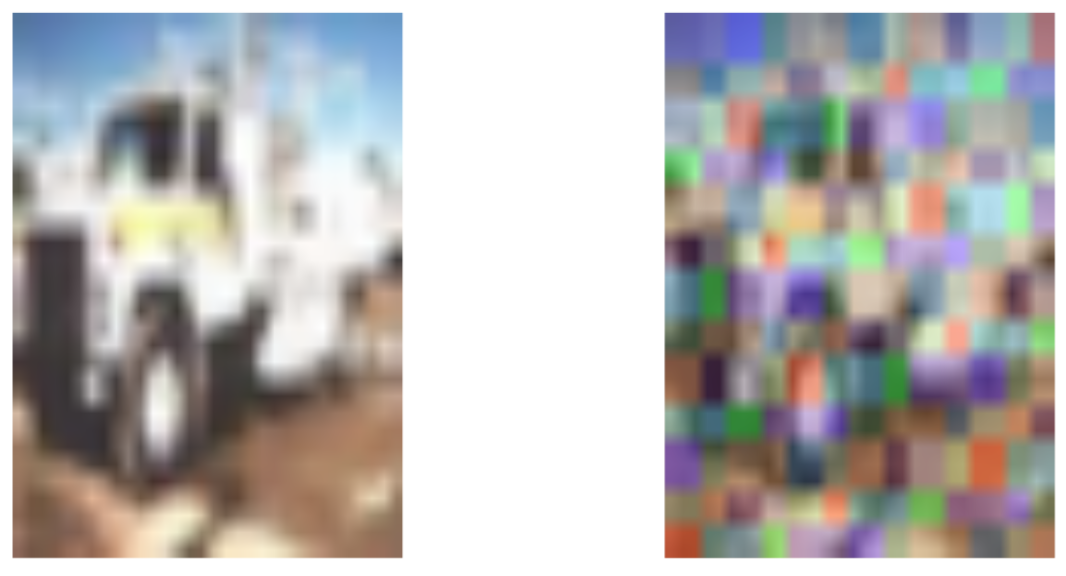
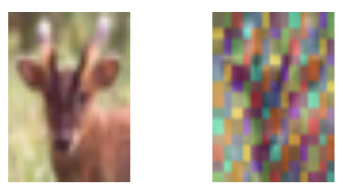
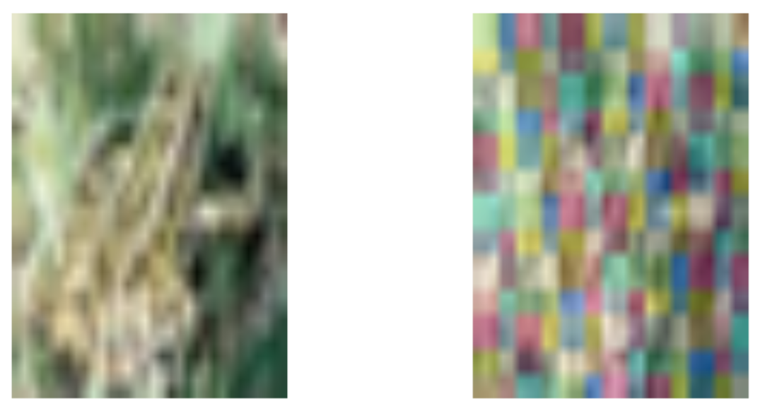
The first case is a deer. We can see that executing Grad CAM overlays three colors, red-blue-green, over the picture. These correspond to the critical regions (that led to the classification decision) for each color. In this case, unsurprisingly, we can see that the ears and the slim face are important image structures. This trends can be seen in all three colors, particularly on the left side of the face. The second case is a frog. We can see that the green color highlights the forg;s forehead, specifically the region around its eye. This makes sense since that is a feature that is fairly unique to the animal. We can also see that the frog’s back leg is highlighted. The third case is a truck. Immediately, a distinct absence of color where the windows are can be noticed. There is color surrounding the front window, yet there is little to none in it. Likely, a defining feature of the truck is its geometric structures, such as a rectangular window. All in all, we can see that Grad CAM offers an interesting perspective into a model that is often regarded as a black box. It intuitively presents the structures it relied on to make its classification decision.
MC Dropout on CNN
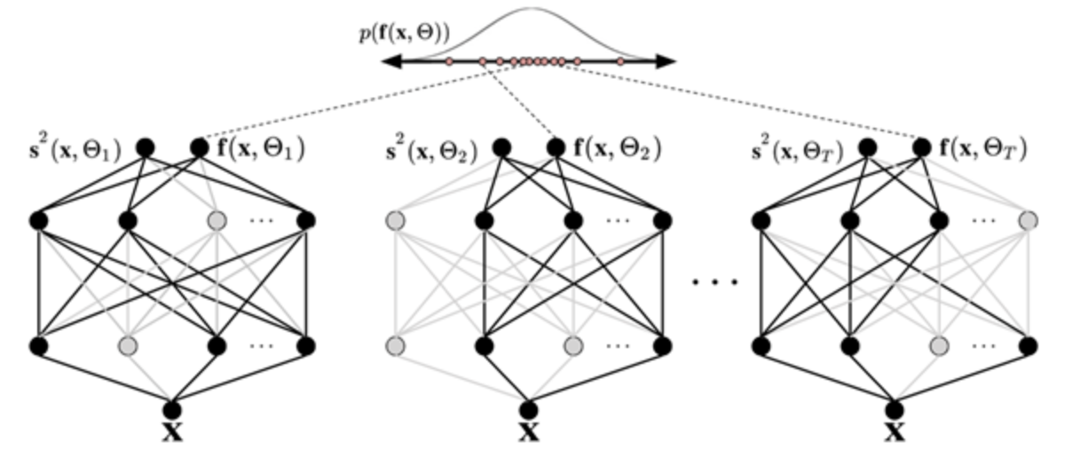
Now, we consider the CNN from section 2 again. MC Dropout enables us to quantify uncertainty in the model’s classification process. Due to limited computing power and time constraints, both the complexity and the samples had to be drastically reduced. MC Dropout implies performing multiple forward passes in a Neural Network, exploiting varying configurations of model architecture to reflect uncertainty in the model’s estimations. In our CNN, we embed the dropout layers into the CNN.
#Data Prep
cat('x_train_shape:', dim(x_train), '\n')
cat(nrow(x_train), 'train samples\n')
cat(nrow(x_test), 'test samples\n')

# Setting up tuning parameters
DropoutRate <- 0.05
tau <- 0.5

keep_prob <- 1-DropoutRate
n_train <- nrow(x_train)
penalty_weight <- keep_prob/(2*tau* n_train)
penalty_intercept <- 1/(2*tau* n_train)

#Setting up drouput from the beginning
dropout_1 <- layer_dropout(rate = DropoutRate)
dropout_2 <- layer_dropout(rate = DropoutRate)

inputs = layer_input(shape = input_shape)

# Define model
output <- inputs %>%
  layer_conv_2d(filters = 32, kernel_size = c(3,3), activation = 'relu') %>%
  layer_max_pooling_2d(pool_size = c(2, 2)) %>%
  layer_conv_2d(filters = 64, kernel_size = c(3,3), activation = 'relu') %>%
  layer_max_pooling_2d(pool_size = c(2, 2)) %>%
  layer_conv_2d(filters = 128, kernel_size = c(3,3), activation = 'relu') %>%
  layer_max_pooling_2d(pool_size = c(2, 2)) %>%
  layer_flatten() %>%
  layer_dense(units = 128, activation = 'relu',
              kernel_regularizer=regularizer_l2(penalty_weight),
              bias_regularizer=regularizer_l2(penalty_intercept)) %>%
  dropout_1(training=TRUE) %>%
  layer_dense(units = 128, activation = 'relu',
              kernel_regularizer=regularizer_l2(penalty_weight),
              bias_regularizer=regularizer_l2(penalty_intercept)) %>%
  dropout_2(training=TRUE) %>%
  layer_dense(units = num_classes, activation = 'softmax')

model <- keras_model(inputs, output)
summary(model)
| Layer (type) | Output Shape | Param # |
|---|---|---|
| input_1 (InputLayer) | (None, 32, 32, 3) | 0 |
| conv2d_4 (Conv2D) | (None, 30, 30, 32) | 896 |
| max_pooling2d_5 | (None, 15, 15, 32) | 0 |
| (MaxPooling2D) | ||
| conv2d_3 (Conv2D) | (None, 13, 13, 64) | 18,496 |
| max_pooling2d_4 | (None, 6, 6, 64) | 0 |
| (MaxPooling2D) | ||
| conv2d_2 (Conv2D) | (None, 4, 4, 128) | 73,856 |
| max_pooling2d_3 | (None, 2, 2, 128) | 0 |
| (MaxPooling2D) | ||
| flatten_1 (Flatten) | (None, 512) | 0 |
| dense_5 (Dense) | (None, 128) | 65,664 |
| dropout_2 (Dropout) | ||
| dense_4 (Dense) | (None, 128) | 16,512 |
| dropout_3 (Dropout) | ||
| dense_3 (Dense) | (None, 3) | 387 |
Total params: 175,811
Trainable params: 175,811
Non-trainable params: 0
#specify optimizer, loss function, metrics
model %>% compile(
  loss = 'categorical_crossentropy',
  optimizer = 'adam',
  metrics = c('accuracy')
)

#set up early stopping
callback_specs=list(callback_early_stopping(monitor = "val_loss", min_delta = 0, patience = 5,
                                            verbose = 0, mode = "auto"),
                    callback_model_checkpoint(filepath='best_model.hdf5',save_freq='epoch' ,save_best_only = TRUE)
)

#running optimization
history <- model %>% fit(
  x_train, y_train,
  epochs = 11, batch_size = 128,
  validation_split = 0.2,
  callbacks = callback_specs
)

#load the saved best model
model_best = load_model_hdf5('best_model.hdf5',compile=FALSE)

#prediction via mcdropout sampling
mc.sample=300 #adjusted to 300 because data are too large
testPredict=array(NA,dim=c(nrow(x_test),3,mc.sample))

for(i in 1:mc.sample){
  testPredict[,,i]=model_best %>%
  predict(x_test)
}

#the true lables
y_true = apply(y_test,1,which.max)

#now each time you compute the predicted values, the results will be slightly different ...
p_hat_test = model_best %>% predict(x_test)
y_hat_test = apply(p_hat_test,1,which.max)

#visualizations for the three categories (Distributions via Boxplot)
mc_plot <- t(testPredict[1,,])
colnames(mc_plot) <- c("Category 1", "Category 2", "Category 3")

boxplot(mc_plot)
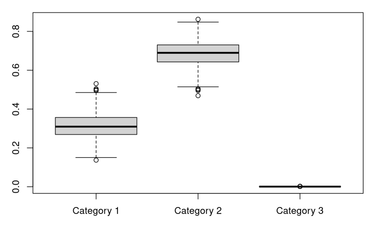
The results show the prediction probability by category (Frogs, Deer, and Trucks). A higher mean corresponds to a higher probability that the model will choose correctly. An ideal result would be close to 1, poor performance would be closer to zero. Anything beyond 33% in this case would be doing worse than a random guess. Using MC Dropout, we can see that the probability of correctly guessing the first category is about 80%. There are outliers below 80%. This excellent performance is contrasted starkly by the other two categories. Cat. 2 is just below 20% and Cat. 3 is at about 0%. All in all, this indicates excellent performance as Cat. 1 classification is very high!
VNN
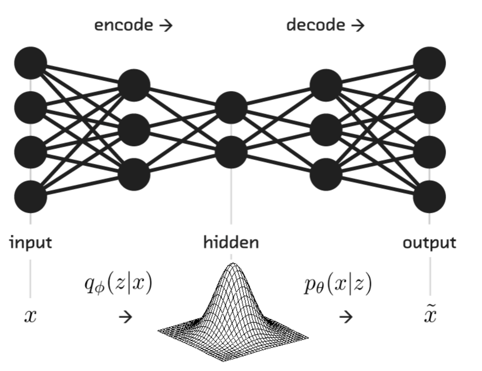
Lastly, we use another approach to quantifying uncertainty: A variational neural network (VNN). A VNN relies on architecture that introduces a random layer (Latent layer “Z”) into the model, enabling the capture of uncertainty.
if (tensorflow::tf$executing_eagerly())
  tensorflow::tf$compat$v1$disable_eager_execution()

# Parameters
batch_size <- 100L
latent_dim <- 3L
intermediate_dim <- 64L
epochs <- 20L
epsilon_std <- 1.0
num_units <- num_classes

# Model definition
x <- layer_input(shape = input_shape)
h <- x %>% layer_conv_2d(filters = 32, kernel_size = c(3,3), activation = "relu") %>%
  layer_max_pooling_2d(pool_size = c(2,2)) %>%
  layer_flatten %>%
  layer_dense(units = 128, activation = 'relu')
z_mean <- layer_dense(h, latent_dim)
z_log_var <- layer_dense(h, latent_dim)

sampling <- function(arg){
  z_mean <- arg[, 1:(latent_dim)]
  z_log_var <- arg[, (latent_dim + 1):(2 * latent_dim)]

  epsilon <- k_random_normal(
    shape = c(k_shape(z_mean)[[1]]),
    mean=0.,
    stddev=epsilon_std
  )

  z_mean + k_exp(z_log_var/2)*epsilon
}

z <- layer_concatenate(list(z_mean, z_log_var)) %>%
  layer_lambda(sampling)

#decoder from Z to Y
decoder_h <- layer_dense(units = intermediate_dim, activation = "relu")
decoder_p <- layer_dense(units = num_units, activation = "softmax")
h_decoded <- decoder_h(z)
y_decoded_p <- decoder_p(h_decoded)

# we instantiate these layers separately so as to reuse them later
# end-to-end variational model
vnn <- keras_model(x, y_decoded_p)

# encoder, from inputs to latent space
encoder <- keras_model(x, z_mean)

vnn_loss <- function(x, x_decoded_mean){
  cat_loss <- loss_categorical_crossentropy(x, x_decoded_mean)
  kl_loss <- -0.5*k_mean(1 + z_log_var - k_square(z_mean) - k_exp(z_log_var), axis = -1L)
  cat_loss + kl_loss
}

vnn %>%
  compile(optimizer = "adam", loss = vnn_loss)

# Model training
vnn %>% fit(
  x_train, y_train,
  shuffle = TRUE,
  epochs = epochs,
  batch_size = batch_size,
  validation_data = list(x_test, y_test)
)

summary(vnn)
| Layer (type) | Output Shape | Param # | Connected to |
|---|---|---|---|
| input_2 (InputLayer) | (None, 32, 32, 3) | 0 | |
| conv2d_5 (Conv2D) | (None, 30, 30, 32) | 896 | |
| max_pooling2d_6 (MaxPooling2D) | (None, 15, 15, 32) | 0 | [] [‘input_2[0][0]’] [‘conv2d_5[0][0]’] |
| flatten_2 (Flatten) | (None, 7200) | 0 | [‘max_pooling2d_6[0][0]’] |
| dense_6 (Dense) | (None, 128) | 921,728 | [‘flatten_2[0][0]’] |
| dense_7 (Dense) | (None, 3) | 387 | [‘dense_6[0][0]’] |
| dense_8 (Dense) | (None, 3) | 387 | [‘dense_6[0][0]’] |
| concatenate (Concatenate) | (None, 6) | 0 | [‘dense_7[0][0]’, ‘dense_8[0][0]’] |
| lambda (Lambda) | (None, 32, 32, 3) | 256 | [‘concatenate[0][0]’] |
| dense_9 (Dense) | (None, 64) | 195 | [‘lambda[0][0]’] |
| dense_10 (Dense) | (None, 3) | 195 | [‘dense_9[0][0]’] |
Total params: 923,849
Trainable params: 923,849
Non-trainable params: 0
# Visualizations for the three categories (Distributions via Boxplot)
library(ggplot2)
library(dplyr)

x_test_decoded<-array(NA,dim=c(nrow(x_test),3,10))
for(i in 1:10){
  x_test_decoded[,,i] <-predict(vnn, x_test)
}

prob_to_plot<-t(x_test_decoded[134,,])
colnames(prob_to_plot) <- c("Category 1", "Category 2", "Category 3")
boxplot(prob_to_plot)

prob_to_plot<-t(x_test_decoded[5,,])
colnames(prob_to_plot) <- c("Category 1", "Category 2", "Category 3")
boxplot(prob_to_plot)
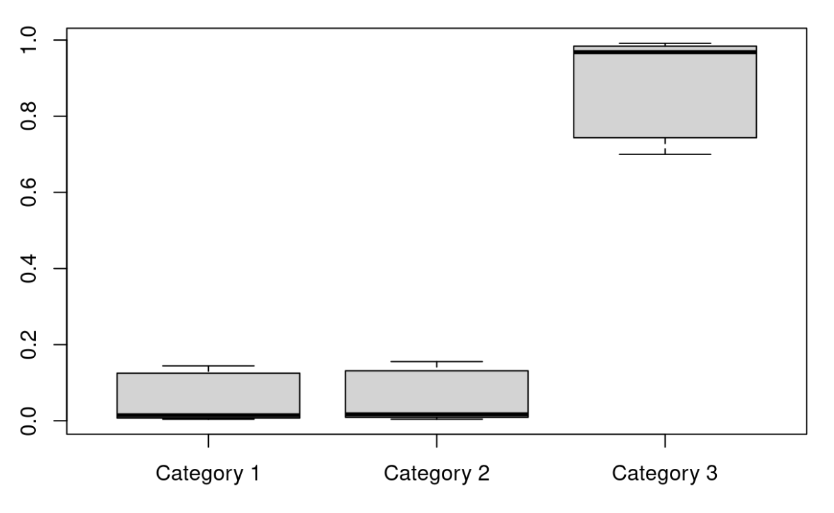
For analysis, we consider two test cases. Both show that within this VNN it is much more likely that categories are incorrectly classified. In both cases, all three categories hover around 33% which indicates poorer classification performance. The distribution of predicted probabilities remains fairly constant across categories.