Inference via Conditional Permutation Tests

Introduction

In hypothesis testing, knowledge about the null distribution is critical. If the null distribution is misspecified, inference may be biased and invalid. In multiple testing scenarios, this vulnerability to misspecification persists. That is why we explore a non-parametric permutation-based approach to multiple testing using conditional permutation tests. The conditional permutation tests–as opposed to a canonical permutation strategy–incorporate covariates into the inferential procedure.

Data and Working Example

As members of the UChicago community, we are aware of occasional safety risks present. The University of Chicago’s administration has responded to these concerns in multiple ways. One of them is offering students up to 10 free Lyft rides per quarter. This has made us curious whether there is a significant association between neighborhood of origin and late night taxi rides. We hypothesize that certain communities in Chicago, especially Hyde Park, are more strongly associated with late night taxi ridership. In our analysis, we account for data from 2014 and 2019. In the following analysis, we will be testing whether there is a relationship between late night rides and over 60 pickup locations, i.e. neighborhoods in Chicago. This results in a multiple testing problem. We generate p-values via (1) a proportion test and (2) via a conditional permutation test, attempting to correct for multiple testing in the latter.

# General wrangling
taxi_df <- taxi_dta %>%
  # Data wrangling
  mutate(year = substr(trip_start_timestamp, 1, 4),
         month = substr(trip_start_timestamp, 6, 7),
         temp = ifelse(month >= '04' & month <= '09', 0, 1),
         pickup_hour = substr(trip_start_timestamp, 12, 13),
         late_ride = ifelse((pickup_hour >= '00' & pickup_hour <= '04') | 
                              (pickup_hour >= '22' & pickup_hour <= '23'), 
                            1, 0)) %>%
  # Filter to 2019
  filter(year == '2014' | year == "2019") %>%
  # Retain only relevant data
  select(pickup_community_area, year, temp, late_ride)

#Filter out pickup locations with less than 1000 data points
  counts = as.data.frame(table((taxi_df[, "pickup_community_area"])))
  counts = counts[!(counts$Freq<1000),]
  taxi_df = taxi_df[(taxi_df$pickup_community_area %in% counts[,1]),]

# Summary Statistics
print(paste0("There are ",length(unique(taxi_df$pickup_community_area))," distinct pickup locations. ",sum(taxi_df$late_ride)*100/nrow(taxi_df),"% of rides are classified as late-night rides."))

Exploratory analysis revealed that multiple communities only have very few ridership data. Thus, we decided to focus only on communities that have more than 1,000 rides. Though it is somewhat arbitrary, we defined a late ride pickup as a taxi ride occuring between 10pm and 4am. Moreover, we controlled for a temperature variable since we are familiar with the harsh Chicago winters. Since no accurate temperature variable is given within the data, we decided to assign a binary cold vs. warm variable to cold and warm months, respectively. We classified September through April as cold months.

Proportion Test

We plan on obtaining p-values in two different ways. First, we obtain p-values by performing a proportion test between 2014 and 2019 late night ride proportions.

# 2014 observations only
prop14_df <- taxi_df %>%
  filter(year == '2014') %>%
  select(pickup_community_area, late_ride) %>%
  group_by(pickup_community_area) %>%
  summarise(late_ride = sum(late_ride), 
            all_ride = n())

# 2019 observations only
prop19_df <- taxi_df %>%
  filter(year == '2019') %>%
  select(pickup_community_area, late_ride) %>%
  group_by(pickup_community_area) %>%
  summarise(late_ride = sum(late_ride), 
            all_ride = n())

# Column bind
prop_df <- merge(prop14_df, prop19_df, 
                 by = "pickup_community_area",
                 suffixes = c("_14", "_19"))

Now, we can perform the proportion test and obtain a vector of p-values.

# Significance Cutoff
alpha = 0.05

# Function to calculate p-values
pvals_prop <- function(df) {
  # Initialize an empty vectors to store p-values
  res <- numeric(nrow(df))
  pvals <- numeric(nrow(df))
  for (i in 1:nrow(df)) {
    # Rowwise proportion test
    res <- prop.test(x = c(df[i,2], df[i,4]), n = c(df[i,3], df[i,5]))
    # Store the p-value in the res vector
    pvals[i] <- res$p.value
  }
  # Return
  return(pvals)
}

# P-values
pvals_prop <- as.data.frame(cbind(prop_df[,1], pvals_prop(prop_df)))

# Histogram
hist(pvals_prop[,2])

# Performance: No correction
print(paste0("When comparing proportions and without any multiple testing correction, ",sum(pvals_prop[,2] < alpha)," out of ",nrow(pvals_prop), " cases have a p-value under the significance cutoff of ", alpha))

The results are indicative of the multiple testing issues present in the data. Our null hypothesis is that there is no relationship between pickup origin and late night ridership. We are testing this null hypothesis against 18 alternative hypothesis. With each statistical test, the probability of obtaining false positives increases. Therefore, we decided to obtain a second set of p-values using a conditional permutation test.

Permutation Test

We now apply a conditional permutation test (CPR) as outlined in Berrett et al., 2018. For us, applying a conditional permutation test is especially useful because we can now test conditional independence, i.e. \(X\) independent from \(Y \vert Z\), rather than just \(X\) independent from \(Y\) as in the previous proportion test. This allows us to account for relevant influence from confounders. Additionally, the conditional permutation test allows us to construct a sampling distribution, rather than assuming it, by resampling combinations of X for each permutation \(X^{(m)}\).

As our test statistic, we have chosen a logistic regression model, regressing late_ride (\(Y\)) on pickup community (\(X\)). Moreover, we control by year and temperature (\(Z\)). We chose a logistic regression model because the dependent variable is binary. Our test statistics, being a function of our data, will output coefficients. We call the non-permuted coefficient vector \(b_T\) and the permuted coefficient vectors \(b_{p_1}, b_{p_2}, ..., b_{p_m}\).

It is noteworthy that computational feasibility prevents us from implementing n!, i.e. 18! = 6.4023737e+15, permutations. Thus, we chose to implement an approximate permutation test with a fixed M large enough to account for a reasonable set of permutations without exceeding a reasonable computational time frame.

# Number of permutations
M = 250

# Isolate X_T 
perm_X <- as.data.frame(taxi_df[,1]) %>%
  rename(X_T = `taxi_df[, 1]`)

# Create a function to permute the data
permute_data <- function(data) {
  return(sample(data, replace = FALSE))
}

# Loop to create M new columns with permuted data
for (i in 1:M) {
  new_col <- permute_data(perm_X$X_T)
  col_name <- paste0("Xp_", i)
  perm_X[col_name] <- new_col
}

# Merge the non-permuted df back
perm_df <- cbind(perm_X, taxi_df[,2:4])

We have obtained a permuted data frame. Let us now turn to the test statistic: A logistic regression model. Note that the logistic regression model only iterates through the M + 1 column vectors of permuted pickup origin. Interestingly, Berrett et al., 2018 propose a slightly different fix if Z is categorical. Namely, “there is a simple and well- known fix for this problem: we can group the observations according to their value of Z, and then permute within groups.” We decided against this approach because our logistic regression model accounts for the conditional dependence. Thus, permuting within each group of \(Z\), i.e. within cold and warm months, would be redundant.

# Create an empty matrix to store the coefficients
coeff_matrix <- 
  matrix(NA, nrow = nrow(pvals_prop) - 1 + 3, # -1 comparison dummy; +3 [intercept term + 2 covariates]
         ncol = M + 1)

# Run a logistic regression model `M + 1` times and store coefficients
for (m in 1:(M+1)) {
  lreg <- glm(late_ride ~ factor(perm_df[,m]) + factor(year) + temp, 
              data = perm_df, 
              family = binomial)
  # Store the coefficients in the matrix
  coeff_matrix[, m] <- as.vector(coef(lreg))
}

# Store coeff_matrix and keep only neighborhoods
coeff_df <- as.data.frame(coeff_matrix) %>%
  slice(-1, -c(n()-2,n())) # keep only neighborhood betas

# Absolute value to coeff_df
coeff_df <- abs(coeff_df)

We know have a matrix that includes coefficients for all neighborhoods across the original data and the permutations. Finally, let us calculate the p-values using Equation (3) from Berrett et al., 2018.

# Significance Cutoff
alpha = 0.05

# Function to calculate p-values
cpt <- function(df) {
  # Numeric shell
  pvals <- numeric(nrow(df))
  # Conditional permutation test
  for (i in 1:nrow(df)){
    pvals[i] <- (1 + (sum(df[i,] >= df[i,1]))) / (1 + ncol(df))
  }
  # Return
  return(pvals)
}

# Calculate p-values
pvals_perm <- cpt(coeff_df)

# Histogram
hist(pvals_perm)

# Performance: Permutation
print(paste0("When applying a permutation test, ", sum(pvals_perm < alpha)," out of ",length(pvals_perm), " cases have a p-value under the significance cutoff of ", alpha))

We can see that the p-values are bunched up at 0 after we have permuted. However, it does seem that the p-values are slightly less extremely bunched up at 0. This is good news because our results remain significant even when we construct a new sampling proportion via permutation.

Visualization

Finally, let us visualize our results. We will visualize the neighborhood-specific p-values from the two tests we performed.

# Read in map
map <- st_read("~/Downloads/boundaries/geo_export_e28691ab-0ce8-47d4-a608-9cf7265ff34a.shp")

# Merge in proportion p-values
map <- merge(map, pvals_prop, 
             by.x = "area_numbe", by.y = "V1", 
             all = TRUE)

# Merge permuted pvals back with neighborhood index
pvals_perm_idx <- c(2,3,4,5,6,7,8,16,22,24,28,32,33,41,56,76,77)
pvals_perm_df <- cbind(pvals_perm_idx, pvals_perm)

# Merge in in permuted p-values
map <- merge(map, pvals_perm_df, 
             by.x = "area_numbe", by.y = "pvals_perm_idx", 
             all = TRUE)

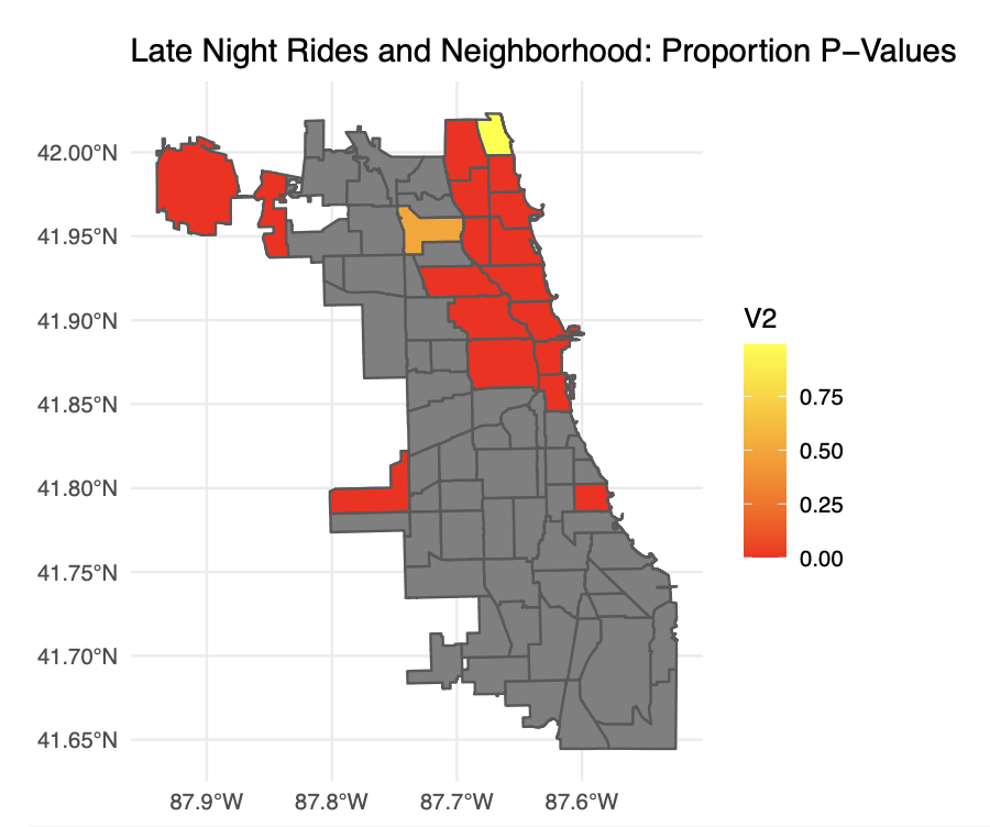
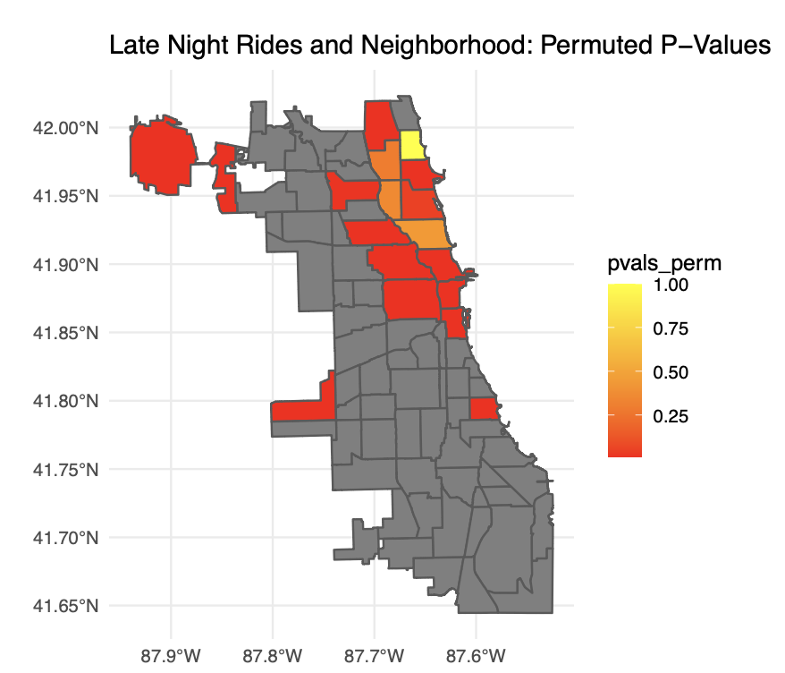
Now, we can contrast our p-values on a neighborhood map. Please note that this visualization does not represent coefficients, but p-values. Thus, these maps should be interpreted as confidence in an association between late night ridership and pickup location.

# Visualization of Proportion P-Values
ggplot() +
  geom_sf(data = map, aes(fill = V2)) +
  scale_fill_gradient(low = "red", high = "yellow") +
  labs(title = "Late Night Rides and Neighborhood: Proportion P-Values") +
  theme_minimal()

# Visualization of Permuted P-Values
ggplot() +
  geom_sf(data = map, aes(fill = pvals_perm)) +
  scale_fill_gradient(low = "red", high = "yellow") +
  labs(title = "Late Night Rides and Neighborhood: Permuted P-Values") +
  theme_minimal()

Overall, both maps tell a story that is not very surprising. As we had hypothesized, Hyde Park is only one of two significant neighborhoods in the South side. The other one is Garfield Ridge, the location of Midway airport. Hyde Park’s significance likely has a lot to do with students taking taxis out of Hyde Park late at night. Furthermore, O’Hare airport is strongly significant. This makes sense since we expect a major international airport to have a lot of late night taxi ridership. Lastly, it is interesting to see that the North Side is very significant, e.g., Lincoln Park and Lakeview. We believe this could be associated with the night life and the comparatively wealthy residents.

Although the differences between the two sets of p-values are small, they are noticeable in the North Side. Some neighborhoods around Lakeview–especially Edgewater and Lincoln Park–become less significant after we conduct the permutation test. This is indicative of the multiple testing correction we performed via permutation.